This blog is a continuation of our Linear Regression blog series. In this part of the blog, we will learn how to estimate the value using the model and compute the error in R.
No Intercept Linear Regression Model and RMSE in R
The essential part of the model code required from our previous blogs is given below:
# Import the file. (File download link)
> inc_exp <- read.csv("Inc_Exp_Data.csv", header=T)

# Variable transformation
> inc_exp$Ln_Emi_or_Rent_Amt = log(inc_exp$Emi_or_Rent_Amt + 1)


# Build Model
> m_linear_mod <- lm(
Mthly_HH_Expense ~ Mthly_HH_Income
+ No_of_Fly_Members + Ln_Emi_or_Rent_Amt,
data = inc_exp
)
> summary(m_linear_mod)$adj.r.squared
[1] 0.7435739


# Predict on Training Set
> expected = predict(m_linear_mod, inc_exp)

> result = as.data.frame(
cbind(
observed = inc_exp$Mthly_HH_Expense,
expected = round(expected))
)
> result$residual = result$observed - result$expected
# Root Mean Squared Error can be interpreted as Standard Deviation of the Residuals (Unexplained Variance).
> rmse = sqrt(mean((result$residual)^2))
> rmse
[1] 5872.303

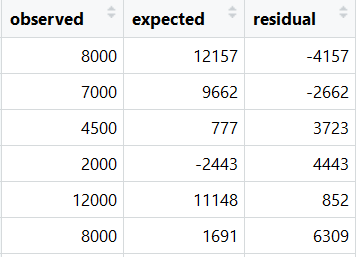
> View(result)

Note: One of the expected values is negative. The estimated values in Linear Regression are not bounded and it can take any value from minus infinity to plus infinity. However, Monthly Household Expense cannot be negative. To overcome this problem, you may have to build a NO INTERCEPT LINEAR REGRESSION MODEL.
No Intercept Linear Regression Model
“No Intercept” regression model is known as fitting a model without an intercept, intercept = 0. It is typically advised to not force the intercept to be 0. You should use No Intercept model only when you are sure that Y = 0 when all X = 0.
R Syntax for No Intercept Model
> no_intercept_mod <- lm(
Mthly_HH_Expense ~ Mthly_HH_Income
+ No_of_Fly_Members + Ln_Emi_or_Rent_Amt + 0,
data = inc_exp
)

summary(no_intercept_mod)$adj.r.squared
[1] 0.911357
Note: The R-Squared of the No Intercept model is more than the R Squared of model with intercept, but keep in mind that the R-Squared of No Intercept Model is computed by assuming the mean of dependent variable is 0. This may not be true and as such the higher value of R-Squared may not give the true picture.
# Predict the expected monthly expense
> expected = predict(no_intercept_mod, inc_exp)

> result = as.data.frame(
cbind(
observed = inc_exp$Mthly_HH_Expense,
expected = round(expected))
)
> result$residual = result$observed - result$expected

> rmse = sqrt(mean((result$residual)^2))
> rmse
[1] 6437.58

View(result)

From results view, we can observe that there are no negative expected values in “No Intercept Model”.
Model Selection

We will give preference to RMSE over Adj. R Squared and as such consider the Intercept Model or Ensemble of both the models. Why?
1. Adj. R-Squared is a relative measure of fit, whereas, RMSE is an absolute measure of fit.
2. R-Squared is in proportion terms and is unitless, where unit of RMSE is the same as unit of dependent variable.
3. Adj. R-Squared in No Intercept Model is computed assuming the mean of dependent variable is equal to 0, which is not true. The mean of dependent variable, i.e. Monthly Expense in our data is 18818.
4. The limitation of Intercept Model is that it is giving negative values for our dependent variable. We may probably use ensemble of No Intercept Model and Intercept Model. If the predicted value of Intercept Model is negative or below a certain minimum threshold, then we may consider the predicted value of No Intercept Model.
Next Blog
In next blog, we will learn about the Linear Regression assumptions. I hope you the student / blog reader would have enjoyed the Linear Regression series so for. Kindly leave you suggestion / comments in the comment section. Moreover, let me know if this model can be further improvised.


Recent Comments